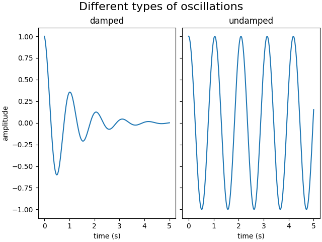
Figurenbezeichnungen: suptitle, supxlabel, supylabel

Jede Achse kann einen Titel haben (eigentlich drei – jeweils mit loc "left", "center" und "right"), aber manchmal ist es wünschenswert, einer ganzen Abbildung (oder einer SubFigure) einen übergeordneten Titel zu geben, mit Figure.suptitle.

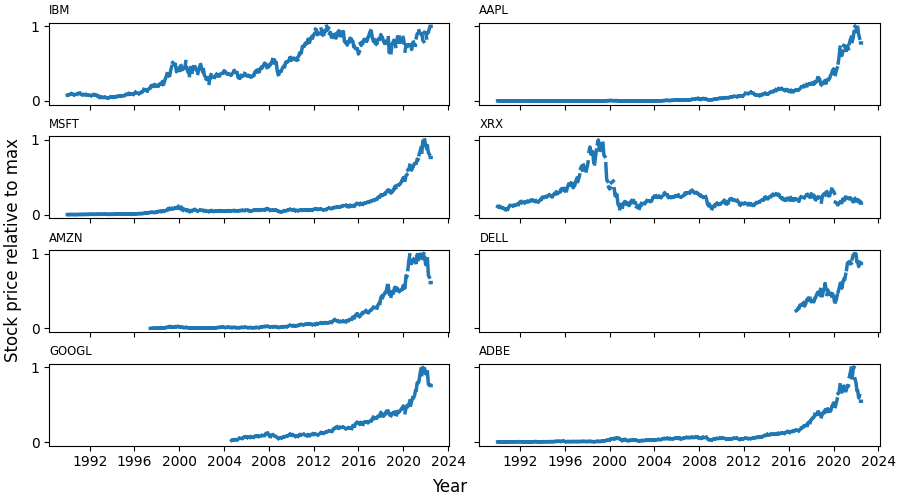
Wir können auch Abbildungs-weite X- und Y-Beschriftungen mit Figure.supxlabel und Figure.supylabel hinzufügen.

import matplotlib.pyplot as plt
import numpy as np

from matplotlib.cbook import get_sample_data

x = np.linspace(0.0, 5.0, 501)

fig, (ax1, ax2) = plt.subplots(1, 2, layout='constrained', sharey=True)
ax1.plot(x, np.cos(6*x) * np.exp(-x))
ax1.set_title('damped')
ax1.set_xlabel('time (s)')
ax1.set_ylabel('amplitude')

ax2.plot(x, np.cos(6*x))
ax2.set_xlabel('time (s)')
ax2.set_title('undamped')

fig.suptitle('Different types of oscillations', fontsize=16)

Eine globale X- oder Y-Beschriftung kann mit den Methoden Figure.supxlabel und Figure.supylabel gesetzt werden.

with get_sample_data('Stocks.csv') as file:
    stocks = np.genfromtxt(
        file, delimiter=',', names=True, dtype=None,
        converters={0: lambda x: np.datetime64(x, 'D')}, skip_header=1)

fig, axs = plt.subplots(4, 2, figsize=(9, 5), layout='constrained',
                        sharex=True, sharey=True)
for nn, ax in enumerate(axs.flat):
    column_name = stocks.dtype.names[1+nn]
    y = stocks[column_name]
    line, = ax.plot(stocks['Date'], y / np.nanmax(y), lw=2.5)
    ax.set_title(column_name, fontsize='small', loc='left')
fig.supxlabel('Year')
fig.supylabel('Stock price relative to max')

plt.show()

Tags: component: figure component: title plot-type: line level: beginner