Schattierungsbeispiel

Beispiel, das zeigt, wie schattierte Reliefdiagramme wie bei Mathematica oder Generic Mapping Tools erstellt werden.

import matplotlib.pyplot as plt
import numpy as np

from matplotlib import cbook
from matplotlib.colors import LightSource


def main():
    # Test data
    x, y = np.mgrid[-5:5:0.05, -5:5:0.05]
    z = 5 * (np.sqrt(x**2 + y**2) + np.sin(x**2 + y**2))

    dem = cbook.get_sample_data('jacksboro_fault_dem.npz')
    elev = dem['elevation']

    fig = compare(z, plt.cm.copper)
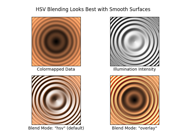
    fig.suptitle('HSV Blending Looks Best with Smooth Surfaces', y=0.95)

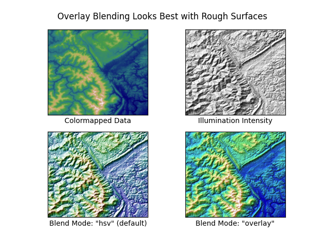
    fig = compare(elev, plt.cm.gist_earth, ve=0.05)
    fig.suptitle('Overlay Blending Looks Best with Rough Surfaces', y=0.95)

    plt.show()


def compare(z, cmap, ve=1):
    # Create subplots and hide ticks
    fig, axs = plt.subplots(ncols=2, nrows=2)
    for ax in axs.flat:
        ax.set(xticks=[], yticks=[])

    # Illuminate the scene from the northwest
    ls = LightSource(azdeg=315, altdeg=45)

    axs[0, 0].imshow(z, cmap=cmap)
    axs[0, 0].set(xlabel='Colormapped Data')

    axs[0, 1].imshow(ls.hillshade(z, vert_exag=ve), cmap='gray')
    axs[0, 1].set(xlabel='Illumination Intensity')

    rgb = ls.shade(z, cmap=cmap, vert_exag=ve, blend_mode='hsv')
    axs[1, 0].imshow(rgb)
    axs[1, 0].set(xlabel='Blend Mode: "hsv" (default)')

    rgb = ls.shade(z, cmap=cmap, vert_exag=ve, blend_mode='overlay')
    axs[1, 1].imshow(rgb)
    axs[1, 1].set(xlabel='Blend Mode: "overlay"')

    return fig


if __name__ == '__main__':
    main()

• 
• 

Referenzen

Die Verwendung der folgenden Funktionen, Methoden, Klassen und Module wird in diesem Beispiel gezeigt

• matplotlib.colors.LightSource

• matplotlib.axes.Axes.imshow / matplotlib.pyplot.imshow