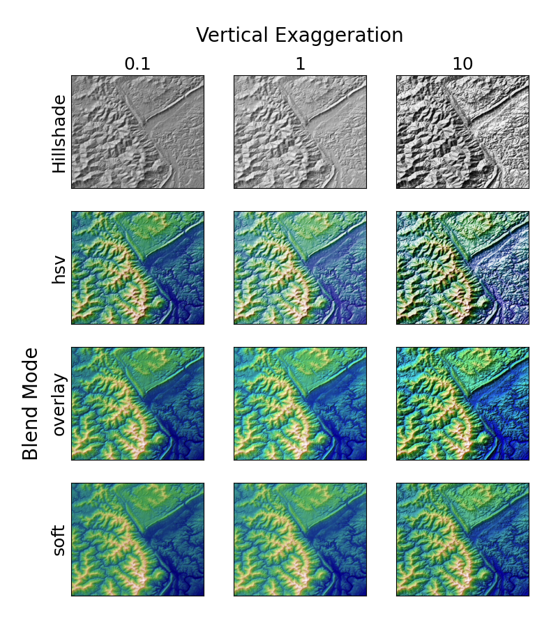
Topographische Neigungs-Schummerung

Demonstriert den visuellen Effekt von variablen Mischmodi und vertikaler Überhöhung bei "neigungsgeschummerten" Plots.

Beachten Sie, dass die Mischmodi "overlay" und "soft" gut für komplexe Oberflächen wie in diesem Beispiel funktionieren, während der Standard-Mischmodus "hsv" am besten für glatte Oberflächen wie viele mathematische Funktionen geeignet ist.

In den meisten Fällen wird die Neigungs-Schummerung rein zu visuellen Zwecken verwendet, und dx/dy können sicher ignoriert werden. In diesem Fall können Sie vert_exag (vertikale Überhöhung) durch Ausprobieren anpassen, um den gewünschten visuellen Effekt zu erzielen. Dieses Beispiel zeigt jedoch, wie die Schlüsselwortargumente dx und dy verwendet werden, um sicherzustellen, dass der Parameter vert_exag die tatsächliche vertikale Überhöhung ist.

import matplotlib.pyplot as plt
import numpy as np

from matplotlib.cbook import get_sample_data
from matplotlib.colors import LightSource

dem = get_sample_data('jacksboro_fault_dem.npz')
z = dem['elevation']
# -- Optional dx and dy for accurate vertical exaggeration --------------------
# If you need topographically accurate vertical exaggeration, or you don't want
# to guess at what *vert_exag* should be, you'll need to specify the cellsize
# of the grid (i.e. the *dx* and *dy* parameters).  Otherwise, any *vert_exag*
# value you specify will be relative to the grid spacing of your input data
# (in other words, *dx* and *dy* default to 1.0, and *vert_exag* is calculated
# relative to those parameters).  Similarly, *dx* and *dy* are assumed to be in
# the same units as your input z-values.  Therefore, we'll need to convert the
# given dx and dy from decimal degrees to meters.
dx, dy = dem['dx'], dem['dy']
dy = 111200 * dy
dx = 111200 * dx * np.cos(np.radians(dem['ymin']))
# -----------------------------------------------------------------------------

# Shade from the northwest, with the sun 45 degrees from horizontal
ls = LightSource(azdeg=315, altdeg=45)
cmap = plt.cm.gist_earth

fig, axs = plt.subplots(nrows=4, ncols=3, figsize=(8, 9))
plt.setp(axs.flat, xticks=[], yticks=[])

# Vary vertical exaggeration and blend mode and plot all combinations
for col, ve in zip(axs.T, [0.1, 1, 10]):
    # Show the hillshade intensity image in the first row
    col[0].imshow(ls.hillshade(z, vert_exag=ve, dx=dx, dy=dy), cmap='gray')

    # Place hillshaded plots with different blend modes in the rest of the rows
    for ax, mode in zip(col[1:], ['hsv', 'overlay', 'soft']):
        rgb = ls.shade(z, cmap=cmap, blend_mode=mode,
                       vert_exag=ve, dx=dx, dy=dy)
        ax.imshow(rgb)

# Label rows and columns
for ax, ve in zip(axs[0], [0.1, 1, 10]):
    ax.set_title(f'{ve}', size=18)
for ax, mode in zip(axs[:, 0], ['Hillshade', 'hsv', 'overlay', 'soft']):
    ax.set_ylabel(mode, size=18)

# Group labels...
axs[0, 1].annotate('Vertical Exaggeration', (0.5, 1), xytext=(0, 30),
                   textcoords='offset points', xycoords='axes fraction',
                   ha='center', va='bottom', size=20)
axs[2, 0].annotate('Blend Mode', (0, 0.5), xytext=(-30, 0),
                   textcoords='offset points', xycoords='axes fraction',
                   ha='right', va='center', size=20, rotation=90)
fig.subplots_adjust(bottom=0.05, right=0.95)

plt.show()