Contour Demo#

Einfache Konturplots, Konturen auf einem Bild mit einer Farbleiste für die Konturen und beschriftete Konturen.

import matplotlib.pyplot as plt
import numpy as np

import matplotlib.cm as cm

delta = 0.025
x = np.arange(-3.0, 3.0, delta)
y = np.arange(-2.0, 2.0, delta)
X, Y = np.meshgrid(x, y)
Z1 = np.exp(-X**2 - Y**2)
Z2 = np.exp(-(X - 1)**2 - (Y - 1)**2)
Z = (Z1 - Z2) * 2

Erstellen Sie einen einfachen Konturplot mit Beschriftungen unter Verwendung von Standardfarben. Das Argument inline von clabel steuert, ob die Beschriftungen über den Liniensegmenten der Kontur gezeichnet werden, wodurch die Linien unter der Beschriftung entfernt werden.

fig, ax = plt.subplots()
CS = ax.contour(X, Y, Z)
ax.clabel(CS, fontsize=10)
ax.set_title('Simplest default with labels')

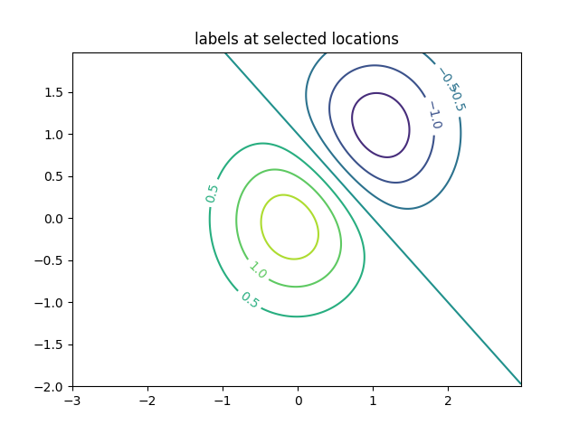
Konturbeschriftungen können manuell platziert werden, indem eine Liste von Positionen (in Datenkoordinaten) angegeben wird. Siehe Interaktive Funktionen für interaktive Platzierung.

fig, ax = plt.subplots()
CS = ax.contour(X, Y, Z)
manual_locations = [
    (-1, -1.4), (-0.62, -0.7), (-2, 0.5), (1.7, 1.2), (2.0, 1.4), (2.4, 1.7)]
ax.clabel(CS, fontsize=10, manual=manual_locations)
ax.set_title('labels at selected locations')

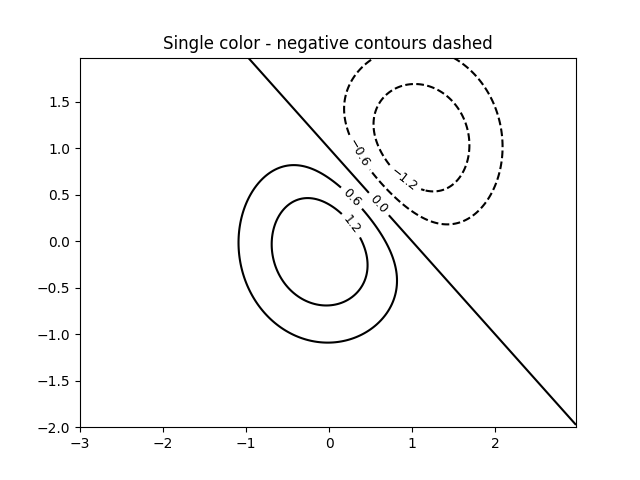
Sie können erzwingen, dass alle Konturen die gleiche Farbe haben.

fig, ax = plt.subplots()
CS = ax.contour(X, Y, Z, 6, colors='k')  # Negative contours default to dashed.
ax.clabel(CS, fontsize=9)
ax.set_title('Single color - negative contours dashed')

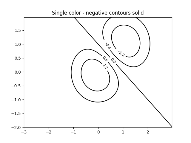
Sie können negative Konturen statt gestrichelt als durchgezogen festlegen

plt.rcParams['contour.negative_linestyle'] = 'solid'
fig, ax = plt.subplots()
CS = ax.contour(X, Y, Z, 6, colors='k')  # Negative contours default to dashed.
ax.clabel(CS, fontsize=9)
ax.set_title('Single color - negative contours solid')

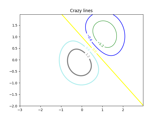
Und Sie können die Farben der Kontur manuell festlegen

fig, ax = plt.subplots()
CS = ax.contour(X, Y, Z, 6,
                linewidths=np.arange(.5, 4, .5),
                colors=('r', 'green', 'blue', (1, 1, 0), '#afeeee', '0.5'),
                )
ax.clabel(CS, fontsize=9)
ax.set_title('Crazy lines')

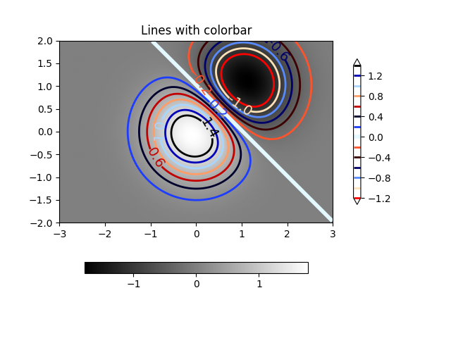
Oder Sie können eine Colormap verwenden, um die Farben festzulegen; die Standard-Colormap wird für die Konturlinien verwendet

fig, ax = plt.subplots()
im = ax.imshow(Z, interpolation='bilinear', origin='lower',
               cmap=cm.gray, extent=(-3, 3, -2, 2))
levels = np.arange(-1.2, 1.6, 0.2)
CS = ax.contour(Z, levels, origin='lower', cmap='flag', extend='both',
                linewidths=2, extent=(-3, 3, -2, 2))

# Thicken the zero contour.
lws = np.resize(CS.get_linewidth(), len(levels))
lws[6] = 4
CS.set_linewidth(lws)

ax.clabel(CS, levels[1::2],  # label every second level
          fmt='%1.1f', fontsize=14)

# make a colorbar for the contour lines
CB = fig.colorbar(CS, shrink=0.8)

ax.set_title('Lines with colorbar')

# We can still add a colorbar for the image, too.
CBI = fig.colorbar(im, orientation='horizontal', shrink=0.8)

# This makes the original colorbar look a bit out of place,
# so let's improve its position.

l, b, w, h = ax.get_position().bounds
ll, bb, ww, hh = CB.ax.get_position().bounds
CB.ax.set_position([ll, b + 0.1*h, ww, h*0.8])

plt.show()

Referenzen

Die Verwendung der folgenden Funktionen, Methoden, Klassen und Module wird in diesem Beispiel gezeigt

Gesamtlaufzeit des Skripts: (0 Minuten 6,386 Sekunden)

Galerie generiert von Sphinx-Gallery