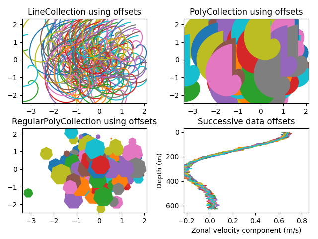
Line, Poly und RegularPoly Collection mit Autoskalierung#

Für die ersten beiden Unterplots verwenden wir Spiralen. Ihre Größe wird in Plot-Einheiten und nicht in Daten-Einheiten festgelegt. Ihre Positionen werden in Daten-Einheiten festgelegt, indem die Schlüsselwortargumente offsets und offset_transform der LineCollection und PolyCollection verwendet werden.

Der dritte Unterplot erstellt regelmäßige Polygone mit der gleichen Art von Skalierung und Positionierung wie in den ersten beiden.

Der letzte Unterplot veranschaulicht die Verwendung von offsets=(xo, yo), d.h. eines einzelnen Tupels anstelle einer Liste von Tupeln, um nacheinander versetzte Kurven zu erzeugen, wobei der Versatz in Daten-Einheiten angegeben ist. Dieses Verhalten ist nur für die LineCollection verfügbar.

import matplotlib.pyplot as plt
import numpy as np

from matplotlib import collections, transforms

nverts = 50
npts = 100

# Make some spirals
r = np.arange(nverts)
theta = np.linspace(0, 2*np.pi, nverts)
xx = r * np.sin(theta)
yy = r * np.cos(theta)
spiral = np.column_stack([xx, yy])

# Fixing random state for reproducibility
rs = np.random.RandomState(19680801)

# Make some offsets
xyo = rs.randn(npts, 2)

# Make a list of colors cycling through the default series.
colors = plt.rcParams['axes.prop_cycle'].by_key()['color']

fig, ((ax1, ax2), (ax3, ax4)) = plt.subplots(2, 2)
fig.subplots_adjust(top=0.92, left=0.07, right=0.97,
                    hspace=0.3, wspace=0.3)


col = collections.LineCollection(
    [spiral], offsets=xyo, offset_transform=ax1.transData)
trans = fig.dpi_scale_trans + transforms.Affine2D().scale(1.0/72.0)
col.set_transform(trans)  # the points to pixels transform
# Note: the first argument to the collection initializer
# must be a list of sequences of (x, y) tuples; we have only
# one sequence, but we still have to put it in a list.
ax1.add_collection(col, autolim=True)
# autolim=True enables autoscaling.  For collections with
# offsets like this, it is neither efficient nor accurate,
# but it is good enough to generate a plot that you can use
# as a starting point.  If you know beforehand the range of
# x and y that you want to show, it is better to set them
# explicitly, leave out the *autolim* keyword argument (or set it to False),
# and omit the 'ax1.autoscale_view()' call below.

# Make a transform for the line segments such that their size is
# given in points:
col.set_color(colors)

ax1.autoscale_view()  # See comment above, after ax1.add_collection.
ax1.set_title('LineCollection using offsets')


# The same data as above, but fill the curves.
col = collections.PolyCollection(
    [spiral], offsets=xyo, offset_transform=ax2.transData)
trans = transforms.Affine2D().scale(fig.dpi/72.0)
col.set_transform(trans)  # the points to pixels transform
ax2.add_collection(col, autolim=True)
col.set_color(colors)


ax2.autoscale_view()
ax2.set_title('PolyCollection using offsets')

# 7-sided regular polygons

col = collections.RegularPolyCollection(
    7, sizes=np.abs(xx) * 10.0, offsets=xyo, offset_transform=ax3.transData)
trans = transforms.Affine2D().scale(fig.dpi / 72.0)
col.set_transform(trans)  # the points to pixels transform
ax3.add_collection(col, autolim=True)
col.set_color(colors)
ax3.autoscale_view()
ax3.set_title('RegularPolyCollection using offsets')


# Simulate a series of ocean current profiles, successively
# offset by 0.1 m/s so that they form what is sometimes called
# a "waterfall" plot or a "stagger" plot.

nverts = 60
ncurves = 20
offs = (0.1, 0.0)

yy = np.linspace(0, 2*np.pi, nverts)
ym = np.max(yy)
xx = (0.2 + (ym - yy) / ym) ** 2 * np.cos(yy - 0.4) * 0.5
segs = []
for i in range(ncurves):
    xxx = xx + 0.02*rs.randn(nverts)
    curve = np.column_stack([xxx, yy * 100])
    segs.append(curve)

col = collections.LineCollection(segs, offsets=offs)
ax4.add_collection(col, autolim=True)
col.set_color(colors)
ax4.autoscale_view()
ax4.set_title('Successive data offsets')
ax4.set_xlabel('Zonal velocity component (m/s)')
ax4.set_ylabel('Depth (m)')
# Reverse the y-axis so depth increases downward
ax4.set_ylim(ax4.get_ylim()[::-1])


plt.show()

LineCollection using offsets, PolyCollection using offsets, RegularPolyCollection using offsets, Successive data offsets

Referenzen

Die Verwendung der folgenden Funktionen, Methoden, Klassen und Module wird in diesem Beispiel gezeigt

Gesamtlaufzeit des Skripts: (0 Minuten 1,293 Sekunden)

Galerie generiert von Sphinx-Gallery