Tripcolor Demo

Pseudofarbenplots von unstrukturierten Dreiecksgittern.

import matplotlib.pyplot as plt
import numpy as np

import matplotlib.tri as tri

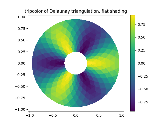
Die Erstellung einer Triangulation ohne Angabe der Dreiecke führt zur Delaunay-Triangulation der Punkte.

# First create the x and y coordinates of the points.
n_angles = 36
n_radii = 8
min_radius = 0.25
radii = np.linspace(min_radius, 0.95, n_radii)

angles = np.linspace(0, 2 * np.pi, n_angles, endpoint=False)
angles = np.repeat(angles[..., np.newaxis], n_radii, axis=1)
angles[:, 1::2] += np.pi / n_angles

x = (radii * np.cos(angles)).flatten()
y = (radii * np.sin(angles)).flatten()
z = (np.cos(radii) * np.cos(3 * angles)).flatten()

# Create the Triangulation; no triangles so Delaunay triangulation created.
triang = tri.Triangulation(x, y)

# Mask off unwanted triangles.
triang.set_mask(np.hypot(x[triang.triangles].mean(axis=1),
                         y[triang.triangles].mean(axis=1))
                < min_radius)

tripcolor-Plot.

fig1, ax1 = plt.subplots()
ax1.set_aspect('equal')
tpc = ax1.tripcolor(triang, z, shading='flat')
fig1.colorbar(tpc)
ax1.set_title('tripcolor of Delaunay triangulation, flat shading')

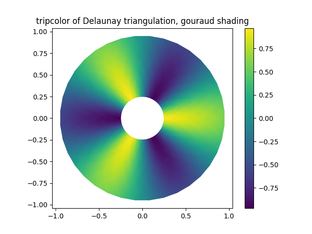
Gouraud-Schattierung veranschaulichen.

fig2, ax2 = plt.subplots()
ax2.set_aspect('equal')
tpc = ax2.tripcolor(triang, z, shading='gouraud')
fig2.colorbar(tpc)
ax2.set_title('tripcolor of Delaunay triangulation, gouraud shading')

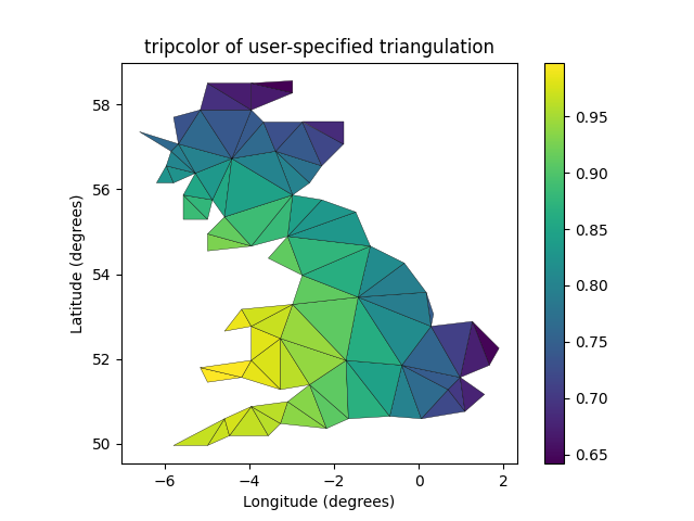
Sie können Ihre eigene Triangulation angeben, anstatt eine Delaunay-Triangulation der Punkte durchzuführen, wobei jedes Dreieck durch die Indizes der drei Punkte gegeben ist, aus denen das Dreieck besteht, geordnet in einem Uhrzeigersinn oder gegen den Uhrzeigersinn.

xy = np.asarray([
    [-0.101, 0.872], [-0.080, 0.883], [-0.069, 0.888], [-0.054, 0.890],
    [-0.045, 0.897], [-0.057, 0.895], [-0.073, 0.900], [-0.087, 0.898],
    [-0.090, 0.904], [-0.069, 0.907], [-0.069, 0.921], [-0.080, 0.919],
    [-0.073, 0.928], [-0.052, 0.930], [-0.048, 0.942], [-0.062, 0.949],
    [-0.054, 0.958], [-0.069, 0.954], [-0.087, 0.952], [-0.087, 0.959],
    [-0.080, 0.966], [-0.085, 0.973], [-0.087, 0.965], [-0.097, 0.965],
    [-0.097, 0.975], [-0.092, 0.984], [-0.101, 0.980], [-0.108, 0.980],
    [-0.104, 0.987], [-0.102, 0.993], [-0.115, 1.001], [-0.099, 0.996],
    [-0.101, 1.007], [-0.090, 1.010], [-0.087, 1.021], [-0.069, 1.021],
    [-0.052, 1.022], [-0.052, 1.017], [-0.069, 1.010], [-0.064, 1.005],
    [-0.048, 1.005], [-0.031, 1.005], [-0.031, 0.996], [-0.040, 0.987],
    [-0.045, 0.980], [-0.052, 0.975], [-0.040, 0.973], [-0.026, 0.968],
    [-0.020, 0.954], [-0.006, 0.947], [ 0.003, 0.935], [ 0.006, 0.926],
    [ 0.005, 0.921], [ 0.022, 0.923], [ 0.033, 0.912], [ 0.029, 0.905],
    [ 0.017, 0.900], [ 0.012, 0.895], [ 0.027, 0.893], [ 0.019, 0.886],
    [ 0.001, 0.883], [-0.012, 0.884], [-0.029, 0.883], [-0.038, 0.879],
    [-0.057, 0.881], [-0.062, 0.876], [-0.078, 0.876], [-0.087, 0.872],
    [-0.030, 0.907], [-0.007, 0.905], [-0.057, 0.916], [-0.025, 0.933],
    [-0.077, 0.990], [-0.059, 0.993]])
x, y = np.rad2deg(xy).T

triangles = np.asarray([
    [67, 66,  1], [65,  2, 66], [ 1, 66,  2], [64,  2, 65], [63,  3, 64],
    [60, 59, 57], [ 2, 64,  3], [ 3, 63,  4], [ 0, 67,  1], [62,  4, 63],
    [57, 59, 56], [59, 58, 56], [61, 60, 69], [57, 69, 60], [ 4, 62, 68],
    [ 6,  5,  9], [61, 68, 62], [69, 68, 61], [ 9,  5, 70], [ 6,  8,  7],
    [ 4, 70,  5], [ 8,  6,  9], [56, 69, 57], [69, 56, 52], [70, 10,  9],
    [54, 53, 55], [56, 55, 53], [68, 70,  4], [52, 56, 53], [11, 10, 12],
    [69, 71, 68], [68, 13, 70], [10, 70, 13], [51, 50, 52], [13, 68, 71],
    [52, 71, 69], [12, 10, 13], [71, 52, 50], [71, 14, 13], [50, 49, 71],
    [49, 48, 71], [14, 16, 15], [14, 71, 48], [17, 19, 18], [17, 20, 19],
    [48, 16, 14], [48, 47, 16], [47, 46, 16], [16, 46, 45], [23, 22, 24],
    [21, 24, 22], [17, 16, 45], [20, 17, 45], [21, 25, 24], [27, 26, 28],
    [20, 72, 21], [25, 21, 72], [45, 72, 20], [25, 28, 26], [44, 73, 45],
    [72, 45, 73], [28, 25, 29], [29, 25, 31], [43, 73, 44], [73, 43, 40],
    [72, 73, 39], [72, 31, 25], [42, 40, 43], [31, 30, 29], [39, 73, 40],
    [42, 41, 40], [72, 33, 31], [32, 31, 33], [39, 38, 72], [33, 72, 38],
    [33, 38, 34], [37, 35, 38], [34, 38, 35], [35, 37, 36]])

xmid = x[triangles].mean(axis=1)
ymid = y[triangles].mean(axis=1)
x0 = -5
y0 = 52
zfaces = np.exp(-0.01 * ((xmid - x0) * (xmid - x0) +
                         (ymid - y0) * (ymid - y0)))

Anstatt ein Triangulation-Objekt zu erstellen, können Sie einfach x, y und Dreiecks-Arrays direkt an tripcolor übergeben. Es wäre besser, ein Triangulation-Objekt zu verwenden, wenn dieselbe Triangulation mehr als einmal verwendet werden soll, um doppelte Berechnungen zu vermeiden. Sie können einen Farbwert pro Fläche und nicht einen pro Punkt angeben, indem Sie das Schlüsselwortargument facecolors verwenden.

fig3, ax3 = plt.subplots()
ax3.set_aspect('equal')
tpc = ax3.tripcolor(x, y, triangles, facecolors=zfaces, edgecolors='k')
fig3.colorbar(tpc)
ax3.set_title('tripcolor of user-specified triangulation')
ax3.set_xlabel('Longitude (degrees)')
ax3.set_ylabel('Latitude (degrees)')

plt.show()

Referenzen

Die Verwendung der folgenden Funktionen, Methoden, Klassen und Module wird in diesem Beispiel gezeigt

• matplotlib.axes.Axes.tripcolor / matplotlib.pyplot.tripcolor

• matplotlib.tri

• matplotlib.tri.Triangulation