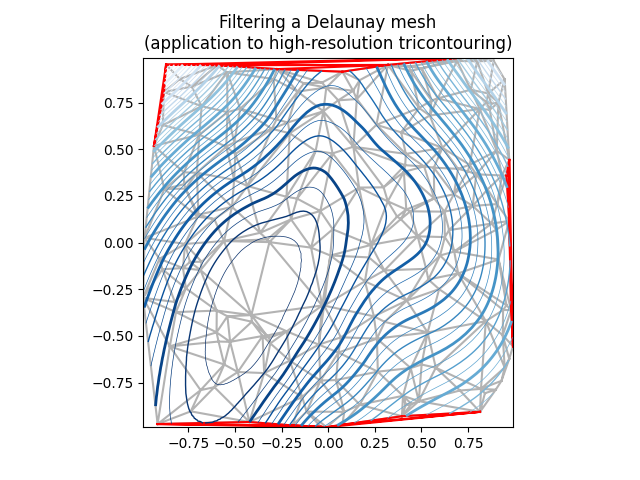
Tricontour Smooth Delaunay#

Demonstriert hochauflösende Tricontouring einer zufälligen Punktmenge; ein matplotlib.tri.TriAnalyzer wird zur Verbesserung der Plotqualität verwendet.

Die anfänglichen Datenpunkte und das Dreiecksgitter für diese Demo sind

eine Menge zufälliger Punkte wird instanziiert, innerhalb des [-1, 1] x [-1, 1] Quadrats
Eine Delaunay-Triangulierung dieser Punkte wird dann berechnet, wobei ein zufälliger Teil der Dreiecke vom Benutzer maskiert wird (basierend auf dem Parameter init_mask_frac). Dies simuliert ungültige Daten.

Das vorgeschlagene generische Verfahren zur Erzielung einer hochauflösenden Konturierung eines solchen Datensatzes ist das folgende:

Berechnen Sie eine erweiterte Maske mit einem matplotlib.tri.TriAnalyzer, der schlecht geformte (flache) Dreiecke vom Rand der Triangulierung ausschließt. Wenden Sie die Maske auf die Triangulierung an (mittels set_mask).
Verfeinern und interpolieren Sie die Daten mit einem matplotlib.tri.UniformTriRefiner.
Plotten Sie die verfeinerten Daten mit tricontour.

import matplotlib.pyplot as plt
import numpy as np

from matplotlib.tri import TriAnalyzer, Triangulation, UniformTriRefiner


# ----------------------------------------------------------------------------
# Analytical test function
# ----------------------------------------------------------------------------
def experiment_res(x, y):
    """An analytic function representing experiment results."""
    x = 2 * x
    r1 = np.sqrt((0.5 - x)**2 + (0.5 - y)**2)
    theta1 = np.arctan2(0.5 - x, 0.5 - y)
    r2 = np.sqrt((-x - 0.2)**2 + (-y - 0.2)**2)
    theta2 = np.arctan2(-x - 0.2, -y - 0.2)
    z = (4 * (np.exp((r1/10)**2) - 1) * 30 * np.cos(3 * theta1) +
         (np.exp((r2/10)**2) - 1) * 30 * np.cos(5 * theta2) +
         2 * (x**2 + y**2))
    return (np.max(z) - z) / (np.max(z) - np.min(z))

# ----------------------------------------------------------------------------
# Generating the initial data test points and triangulation for the demo
# ----------------------------------------------------------------------------
# User parameters for data test points

# Number of test data points, tested from 3 to 5000 for subdiv=3
n_test = 200

# Number of recursive subdivisions of the initial mesh for smooth plots.
# Values >3 might result in a very high number of triangles for the refine
# mesh: new triangles numbering = (4**subdiv)*ntri
subdiv = 3

# Float > 0. adjusting the proportion of (invalid) initial triangles which will
# be masked out. Enter 0 for no mask.
init_mask_frac = 0.0

# Minimum circle ratio - border triangles with circle ratio below this will be
# masked if they touch a border. Suggested value 0.01; use -1 to keep all
# triangles.
min_circle_ratio = .01

# Random points
random_gen = np.random.RandomState(seed=19680801)
x_test = random_gen.uniform(-1., 1., size=n_test)
y_test = random_gen.uniform(-1., 1., size=n_test)
z_test = experiment_res(x_test, y_test)

# meshing with Delaunay triangulation
tri = Triangulation(x_test, y_test)
ntri = tri.triangles.shape[0]

# Some invalid data are masked out
mask_init = np.zeros(ntri, dtype=bool)
masked_tri = random_gen.randint(0, ntri, int(ntri * init_mask_frac))
mask_init[masked_tri] = True
tri.set_mask(mask_init)


# ----------------------------------------------------------------------------
# Improving the triangulation before high-res plots: removing flat triangles
# ----------------------------------------------------------------------------
# masking badly shaped triangles at the border of the triangular mesh.
mask = TriAnalyzer(tri).get_flat_tri_mask(min_circle_ratio)
tri.set_mask(mask)

# refining the data
refiner = UniformTriRefiner(tri)
tri_refi, z_test_refi = refiner.refine_field(z_test, subdiv=subdiv)

# analytical 'results' for comparison
z_expected = experiment_res(tri_refi.x, tri_refi.y)

# for the demo: loading the 'flat' triangles for plot
flat_tri = Triangulation(x_test, y_test)
flat_tri.set_mask(~mask)


# ----------------------------------------------------------------------------
# Now the plots
# ----------------------------------------------------------------------------
# User options for plots
plot_tri = True          # plot of base triangulation
plot_masked_tri = True   # plot of excessively flat excluded triangles
plot_refi_tri = False    # plot of refined triangulation
plot_expected = False    # plot of analytical function values for comparison


# Graphical options for tricontouring
levels = np.arange(0., 1., 0.025)

fig, ax = plt.subplots()
ax.set_aspect('equal')
ax.set_title("Filtering a Delaunay mesh\n"
             "(application to high-resolution tricontouring)")

# 1) plot of the refined (computed) data contours:
ax.tricontour(tri_refi, z_test_refi, levels=levels, cmap='Blues',
              linewidths=[2.0, 0.5, 1.0, 0.5])
# 2) plot of the expected (analytical) data contours (dashed):
if plot_expected:
    ax.tricontour(tri_refi, z_expected, levels=levels, cmap='Blues',
                  linestyles='--')
# 3) plot of the fine mesh on which interpolation was done:
if plot_refi_tri:
    ax.triplot(tri_refi, color='0.97')
# 4) plot of the initial 'coarse' mesh:
if plot_tri:
    ax.triplot(tri, color='0.7')
# 4) plot of the unvalidated triangles from naive Delaunay Triangulation:
if plot_masked_tri:
    ax.triplot(flat_tri, color='red')

plt.show()

Filtering a Delaunay mesh (application to high-resolution tricontouring)

Referenzen

Die Verwendung der folgenden Funktionen, Methoden, Klassen und Module wird in diesem Beispiel gezeigt

Gesamtlaufzeit des Skripts: (0 Minuten 1,725 Sekunden)

Galerie generiert von Sphinx-Gallery