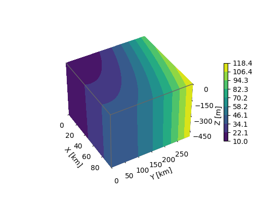
3D Box-Oberflächenplot

Für gegebene Daten in einem gegitterten Volumen X, Y, Z plottet dieses Beispiel die Datenwerte auf den Oberflächen des Volumens.

Die Strategie besteht darin, die Daten von jeder Oberfläche auszuwählen und Konturen separat mithilfe von axes3d.Axes3D.contourf mit den entsprechenden Parametern zdir und offset zu plotten.

import matplotlib.pyplot as plt
import numpy as np

# Define dimensions
Nx, Ny, Nz = 100, 300, 500
X, Y, Z = np.meshgrid(np.arange(Nx), np.arange(Ny), -np.arange(Nz))

# Create fake data
data = (((X+100)**2 + (Y-20)**2 + 2*Z)/1000+1)

kw = {
    'vmin': data.min(),
    'vmax': data.max(),
    'levels': np.linspace(data.min(), data.max(), 10),
}

# Create a figure with 3D ax
fig = plt.figure(figsize=(5, 4))
ax = fig.add_subplot(111, projection='3d')

# Plot contour surfaces
_ = ax.contourf(
    X[:, :, 0], Y[:, :, 0], data[:, :, 0],
    zdir='z', offset=0, **kw
)
_ = ax.contourf(
    X[0, :, :], data[0, :, :], Z[0, :, :],
    zdir='y', offset=0, **kw
)
C = ax.contourf(
    data[:, -1, :], Y[:, -1, :], Z[:, -1, :],
    zdir='x', offset=X.max(), **kw
)
# --


# Set limits of the plot from coord limits
xmin, xmax = X.min(), X.max()
ymin, ymax = Y.min(), Y.max()
zmin, zmax = Z.min(), Z.max()
ax.set(xlim=[xmin, xmax], ylim=[ymin, ymax], zlim=[zmin, zmax])

# Plot edges
edges_kw = dict(color='0.4', linewidth=1, zorder=1e3)
ax.plot([xmax, xmax], [ymin, ymax], 0, **edges_kw)
ax.plot([xmin, xmax], [ymin, ymin], 0, **edges_kw)
ax.plot([xmax, xmax], [ymin, ymin], [zmin, zmax], **edges_kw)

# Set labels and zticks
ax.set(
    xlabel='X [km]',
    ylabel='Y [km]',
    zlabel='Z [m]',
    zticks=[0, -150, -300, -450],
)

# Set zoom and angle view
ax.view_init(40, -30, 0)
ax.set_box_aspect(None, zoom=0.9)

# Colorbar
fig.colorbar(C, ax=ax, fraction=0.02, pad=0.1, label='Name [units]')

# Show Figure
plt.show()

Schlagwörter: plot-type: 3D level: intermediate