Erstellen einer Colormap aus einer Liste von Farben#

Weitere Details zum Erstellen und Manipulieren von Colormaps finden Sie unter Erstellen von Colormaps in Matplotlib.

Das Erstellen einer Colormap aus einer Liste von Farben kann mit der Methode LinearSegmentedColormap.from_list erfolgen. Sie müssen eine Liste von RGB-Tupeln übergeben, die die Mischung der Farben von 0 bis 1 definieren.

Erstellen benutzerdefinierter Colormaps#

Es ist auch möglich, eine benutzerdefinierte Zuordnung für eine Colormap zu erstellen. Dies geschieht durch Erstellen eines Wörterbuchs, das angibt, wie sich die RGB-Kanäle von einem Ende der Colormap zum anderen ändern.

Beispiel: Angenommen, Sie möchten, dass Rot über die untere Hälfte von 0 auf 1 ansteigt, Grün über die mittlere Hälfte dasselbe tut und Blau über die obere Hälfte. Dann würden Sie verwenden

cdict = {
    'red': (
        (0.0,  0.0, 0.0),
        (0.5,  1.0, 1.0),
        (1.0,  1.0, 1.0),
    ),
    'green': (
        (0.0,  0.0, 0.0),
        (0.25, 0.0, 0.0),
        (0.75, 1.0, 1.0),
        (1.0,  1.0, 1.0),
    ),
    'blue': (
        (0.0,  0.0, 0.0),
        (0.5,  0.0, 0.0),
        (1.0,  1.0, 1.0),
    )
}

Wenn, wie in diesem Beispiel, keine Diskontinuitäten in den r-, g- und b-Komponenten vorhanden sind, dann ist es ganz einfach: Das zweite und dritte Element jedes Tupels oben ist dasselbe – nennen wir es "y". Das erste Element ("x") definiert Interpolationsintervalle über den gesamten Bereich von 0 bis 1 und muss diesen gesamten Bereich abdecken. Mit anderen Worten, die Werte von x teilen den Bereich von 0 bis 1 in eine Reihe von Segmenten auf, und y gibt die Endfarbwerte für jedes Segment an.

Betrachten wir nun das Grün, cdict['green'] besagt, dass für

0 <= x <= 0.25, y Null ist; kein Grün.
0.25 < x <= 0.75, y variiert linear von 0 bis 1.
0.75 < x <= 1, y bleibt bei 1, volles Grün.

Wenn Diskontinuitäten vorhanden sind, ist es etwas komplizierter. Beschriften Sie die 3 Elemente in jeder Zeile im cdict-Eintrag für eine bestimmte Farbe als (x, y0, y1). Dann wird für Werte von x zwischen x[i] und x[i+1] die Farbe zwischen y1[i] und y0[i+1] interpoliert.

Zurück zu einem Kochbuch-Beispiel

cdict = {
    'red': (
        (0.0,  0.0, 0.0),
        (0.5,  1.0, 0.7),
        (1.0,  1.0, 1.0),
    ),
    'green': (
        (0.0,  0.0, 0.0),
        (0.5,  1.0, 0.0),
        (1.0,  1.0, 1.0),
    ),
    'blue': (
        (0.0,  0.0, 0.0),
        (0.5,  0.0, 0.0),
        (1.0,  1.0, 1.0),
    )
}

und schauen Sie sich cdict['red'][1] an; da y0 != y1, besagt es, dass für x von 0 bis 0.5 Rot von 0 auf 1 ansteigt, dann aber abspringt, sodass für x von 0.5 bis 1 Rot von 0.7 auf 1 ansteigt. Grün steigt von 0 auf 1 an, wenn x von 0 bis 0.5 geht, springt dann zurück auf 0 und steigt wieder auf 1 an, wenn x von 0.5 bis 1 geht.

row i:   x  y0  y1
               /
              /
row i+1: x  y0  y1

Oben ist ein Versuch zu zeigen, dass für x im Bereich von x[i] bis x[i+1] die Interpolation zwischen y1[i] und y0[i+1] erfolgt. Daher werden y0[0] und y1[-1] nie verwendet.

import matplotlib.pyplot as plt
import numpy as np

import matplotlib as mpl
from matplotlib.colors import LinearSegmentedColormap

# Make some illustrative fake data:

x = np.arange(0, np.pi, 0.1)
y = np.arange(0, 2 * np.pi, 0.1)
X, Y = np.meshgrid(x, y)
Z = np.cos(X) * np.sin(Y) * 10

Colormaps aus einer Liste#

colors = [(1, 0, 0), (0, 1, 0), (0, 0, 1)]  # R -> G -> B
n_bins = [3, 6, 10, 100]  # Discretizes the interpolation into bins
cmap_name = 'my_list'
fig, axs = plt.subplots(2, 2, figsize=(6, 9))
fig.subplots_adjust(left=0.02, bottom=0.06, right=0.95, top=0.94, wspace=0.05)
for n_bin, ax in zip(n_bins, axs.flat):
    # Create the colormap
    cmap = LinearSegmentedColormap.from_list(cmap_name, colors, N=n_bin)
    # Fewer bins will result in "coarser" colomap interpolation
    im = ax.imshow(Z, origin='lower', cmap=cmap)
    ax.set_title("N bins: %s" % n_bin)
    fig.colorbar(im, ax=ax)

N bins: 3, N bins: 6, N bins: 10, N bins: 100

Benutzerdefinierte Colormaps#

cdict1 = {
    'red': (
        (0.0, 0.0, 0.0),
        (0.5, 0.0, 0.1),
        (1.0, 1.0, 1.0),
    ),
    'green': (
        (0.0, 0.0, 0.0),
        (1.0, 0.0, 0.0),
    ),
    'blue': (
        (0.0, 0.0, 1.0),
        (0.5, 0.1, 0.0),
        (1.0, 0.0, 0.0),
    )
}

cdict2 = {
    'red': (
        (0.0, 0.0, 0.0),
        (0.5, 0.0, 1.0),
        (1.0, 0.1, 1.0),
    ),
    'green': (
        (0.0, 0.0, 0.0),
        (1.0, 0.0, 0.0),
    ),
    'blue': (
        (0.0, 0.0, 0.1),
        (0.5, 1.0, 0.0),
        (1.0, 0.0, 0.0),
    )
}

cdict3 = {
    'red': (
        (0.0, 0.0, 0.0),
        (0.25, 0.0, 0.0),
        (0.5, 0.8, 1.0),
        (0.75, 1.0, 1.0),
        (1.0, 0.4, 1.0),
    ),
    'green': (
        (0.0, 0.0, 0.0),
        (0.25, 0.0, 0.0),
        (0.5, 0.9, 0.9),
        (0.75, 0.0, 0.0),
        (1.0, 0.0, 0.0),
    ),
    'blue': (
        (0.0, 0.0, 0.4),
        (0.25, 1.0, 1.0),
        (0.5, 1.0, 0.8),
        (0.75, 0.0, 0.0),
        (1.0, 0.0, 0.0),
    )
}

# Make a modified version of cdict3 with some transparency
# in the middle of the range.
cdict4 = {
    **cdict3,
    'alpha': (
        (0.0, 1.0, 1.0),
        # (0.25, 1.0, 1.0),
        (0.5, 0.3, 0.3),
        # (0.75, 1.0, 1.0),
        (1.0, 1.0, 1.0),
    ),
}

Nun werden wir dieses Beispiel verwenden, um 2 Möglichkeiten zur Handhabung benutzerdefinierter Colormaps zu veranschaulichen. Erstens, die direkteste und expliziteste

blue_red1 = LinearSegmentedColormap('BlueRed1', cdict1)

Zweitens, erstellen Sie die Map explizit und registrieren Sie sie. Wie die erste Methode funktioniert auch diese Methode mit jeder Art von Colormap, nicht nur mit einer LinearSegmentedColormap

mpl.colormaps.register(LinearSegmentedColormap('BlueRed2', cdict2))
mpl.colormaps.register(LinearSegmentedColormap('BlueRed3', cdict3))
mpl.colormaps.register(LinearSegmentedColormap('BlueRedAlpha', cdict4))

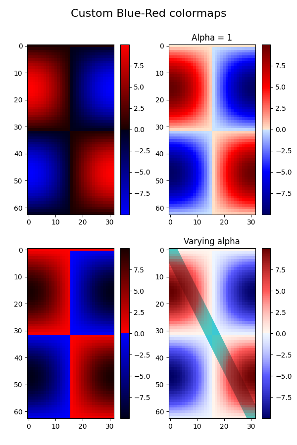
Erstellen Sie die Figur mit 4 Unterplots

fig, axs = plt.subplots(2, 2, figsize=(6, 9))
fig.subplots_adjust(left=0.02, bottom=0.06, right=0.95, top=0.94, wspace=0.05)

im1 = axs[0, 0].imshow(Z, cmap=blue_red1)
fig.colorbar(im1, ax=axs[0, 0])

im2 = axs[1, 0].imshow(Z, cmap='BlueRed2')
fig.colorbar(im2, ax=axs[1, 0])

# Now we will set the third cmap as the default.  One would
# not normally do this in the middle of a script like this;
# it is done here just to illustrate the method.

plt.rcParams['image.cmap'] = 'BlueRed3'

im3 = axs[0, 1].imshow(Z)
fig.colorbar(im3, ax=axs[0, 1])
axs[0, 1].set_title("Alpha = 1")

# Or as yet another variation, we can replace the rcParams
# specification *before* the imshow with the following *after*
# imshow.
# This sets the new default *and* sets the colormap of the last
# image-like item plotted via pyplot, if any.
#

# Draw a line with low zorder so it will be behind the image.
axs[1, 1].plot([0, 10 * np.pi], [0, 20 * np.pi], color='c', lw=20, zorder=-1)

im4 = axs[1, 1].imshow(Z)
fig.colorbar(im4, ax=axs[1, 1])

# Here it is: changing the colormap for the current image and its
# colorbar after they have been plotted.
im4.set_cmap('BlueRedAlpha')
axs[1, 1].set_title("Varying alpha")

fig.suptitle('Custom Blue-Red colormaps', fontsize=16)
fig.subplots_adjust(top=0.9)

plt.show()

Custom Blue-Red colormaps, Alpha = 1, Varying alpha

Referenzen

Die Verwendung der folgenden Funktionen, Methoden, Klassen und Module wird in diesem Beispiel gezeigt

Tags: Styling: Colormap Plot-Typ: imshow Level: Intermediate

Gesamtlaufzeit des Skripts: (0 Minuten 2,105 Sekunden)

Galerie generiert von Sphinx-Gallery