Diagramme annotieren

Die folgenden Beispiele zeigen Möglichkeiten, Diagramme in Matplotlib zu annotieren. Dies beinhaltet die Hervorhebung spezifischer Punkte von Interesse und die Verwendung verschiedener visueller Werkzeuge, um auf diesen Punkt aufmerksam zu machen. Für eine vollständigere und eingehendere Beschreibung der Annotations- und Textwerkzeuge in Matplotlib siehe das Tutorial zur Annotation.

import matplotlib.pyplot as plt
import numpy as np

from matplotlib.patches import Ellipse
from matplotlib.text import OffsetFrom

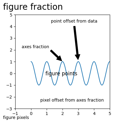
Festlegen von Textpunkten und Annotationspunkten

Sie müssen einen Annotationspunkt xy=(x, y) angeben, um diesen Punkt zu annotieren. Zusätzlich können Sie einen Textpunkt xytext=(x, y) für die Position des Textes für diese Annotation angeben. Optional können Sie das Koordinatensystem von xy und xytext mit einer der folgenden Zeichenfolgen für xycoords und textcoords angeben (Standard ist 'data').

'figure points'   : points from the lower left corner of the figure
'figure pixels'   : pixels from the lower left corner of the figure
'figure fraction' : (0, 0) is lower left of figure and (1, 1) is upper right
'axes points'     : points from lower left corner of the Axes
'axes pixels'     : pixels from lower left corner of the Axes
'axes fraction'   : (0, 0) is lower left of Axes and (1, 1) is upper right
'offset points'   : Specify an offset (in points) from the xy value
'offset pixels'   : Specify an offset (in pixels) from the xy value
'data'            : use the Axes data coordinate system

Hinweis: Für physikalische Koordinatensysteme (Punkte oder Pixel) ist der Ursprung die (untere, linke) Ecke der Abbildung oder der Achsen.

Optional können Sie Pfeileigenschaften angeben, die einen Pfeil vom Text zum annotierten Punkt zeichnen, indem Sie ein Dictionary von Pfeileigenschaften übergeben.

Gültige Schlüssel sind

width : the width of the arrow in points
frac  : the fraction of the arrow length occupied by the head
headwidth : the width of the base of the arrow head in points
shrink : move the tip and base some percent away from the
         annotated point and text
any key for matplotlib.patches.polygon  (e.g., facecolor)

# Create our figure and data we'll use for plotting
fig, ax = plt.subplots(figsize=(4, 4))

t = np.arange(0.0, 5.0, 0.01)
s = np.cos(2*np.pi*t)

# Plot a line and add some simple annotations
line, = ax.plot(t, s)
ax.annotate('figure pixels',
            xy=(10, 10), xycoords='figure pixels')
ax.annotate('figure points',
            xy=(107, 110), xycoords='figure points',
            fontsize=12)
ax.annotate('figure fraction',
            xy=(.025, .975), xycoords='figure fraction',
            horizontalalignment='left', verticalalignment='top',
            fontsize=20)

# The following examples show off how these arrows are drawn.

ax.annotate('point offset from data',
            xy=(3, 1), xycoords='data',
            xytext=(-10, 90), textcoords='offset points',
            arrowprops=dict(facecolor='black', shrink=0.05),
            horizontalalignment='center', verticalalignment='bottom')

ax.annotate('axes fraction',
            xy=(2, 1), xycoords='data',
            xytext=(0.36, 0.68), textcoords='axes fraction',
            arrowprops=dict(facecolor='black', shrink=0.05),
            horizontalalignment='right', verticalalignment='top')

# You may also use negative points or pixels to specify from (right, top).
# E.g., (-10, 10) is 10 points to the left of the right side of the Axes and 10
# points above the bottom

ax.annotate('pixel offset from axes fraction',
            xy=(1, 0), xycoords='axes fraction',
            xytext=(-20, 20), textcoords='offset pixels',
            horizontalalignment='right',
            verticalalignment='bottom')

ax.set(xlim=(-1, 5), ylim=(-3, 5))

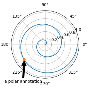
Verwenden mehrerer Koordinatensysteme und Achsentypen

Sie können den xypunkt und den xytext an verschiedenen Positionen und in verschiedenen Koordinatensystemen angeben und optional eine Verbindungslinie einschalten und den Punkt mit einem Marker markieren. Annotationen funktionieren auch auf polaren Achsen.

Im folgenden Beispiel befindet sich der xy-Punkt in nativen Koordinaten (xycoords ist standardmäßig 'data'). Für eine polare Achse ist dies im (theta, radius)-Raum. Der Text im Beispiel wird im fraktionellen Abbildungskoordinatensystem platziert. Text-Schlüsselwörter wie horizontale und vertikale Ausrichtung werden berücksichtigt.

fig, ax = plt.subplots(subplot_kw=dict(projection='polar'), figsize=(3, 3))
r = np.arange(0, 1, 0.001)
theta = 2*2*np.pi*r
line, = ax.plot(theta, r)

ind = 800
thisr, thistheta = r[ind], theta[ind]
ax.plot([thistheta], [thisr], 'o')
ax.annotate('a polar annotation',
            xy=(thistheta, thisr),  # theta, radius
            xytext=(0.05, 0.05),    # fraction, fraction
            textcoords='figure fraction',
            arrowprops=dict(facecolor='black', shrink=0.05),
            horizontalalignment='left',
            verticalalignment='bottom')

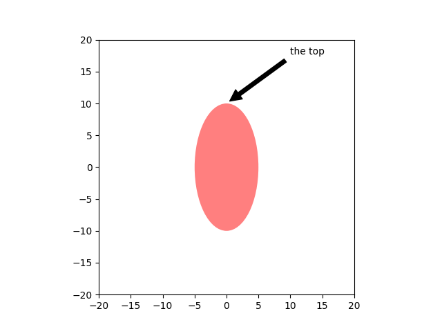
Sie können auch die Polarkoordinatenschreibweise auf einer kartesischen Achse verwenden. Hier ist das native Koordinatensystem ('data') kartesisch, daher müssen Sie xycoords und textcoords als 'polar' angeben, wenn Sie (theta, radius) verwenden möchten.

el = Ellipse((0, 0), 10, 20, facecolor='r', alpha=0.5)

fig, ax = plt.subplots(subplot_kw=dict(aspect='equal'))
ax.add_artist(el)
el.set_clip_box(ax.bbox)
ax.annotate('the top',
            xy=(np.pi/2., 10.),      # theta, radius
            xytext=(np.pi/3, 20.),   # theta, radius
            xycoords='polar',
            textcoords='polar',
            arrowprops=dict(facecolor='black', shrink=0.05),
            horizontalalignment='left',
            verticalalignment='bottom',
            clip_on=True)  # clip to the Axes bounding box

ax.set(xlim=[-20, 20], ylim=[-20, 20])

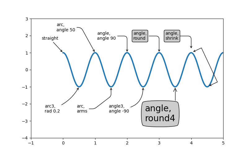
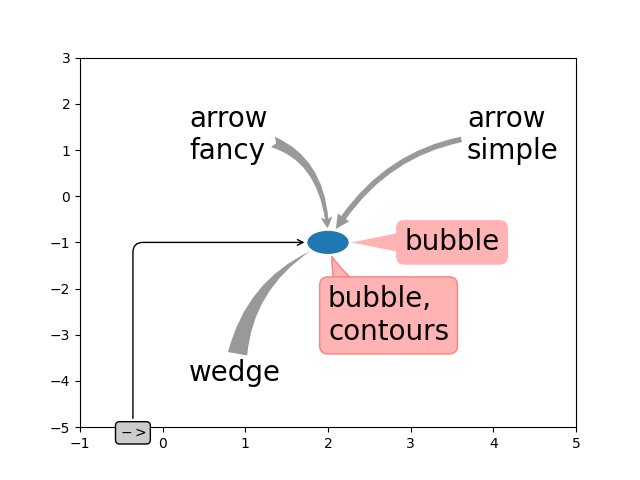
Anpassen von Pfeil- und Sprechblasenstilen

Der Pfeil zwischen xytext und dem Annotationspunkt sowie die Sprechblase, die den Annotationstext umschließt, sind hochgradig anpassbar. Nachfolgend sind einige Parameteroptionen und ihre Ergebnisse aufgeführt.

fig, ax = plt.subplots(figsize=(8, 5))

t = np.arange(0.0, 5.0, 0.01)
s = np.cos(2*np.pi*t)
line, = ax.plot(t, s, lw=3)

ax.annotate(
    'straight',
    xy=(0, 1), xycoords='data',
    xytext=(-50, 30), textcoords='offset points',
    arrowprops=dict(arrowstyle="->"))
ax.annotate(
    'arc3,\nrad 0.2',
    xy=(0.5, -1), xycoords='data',
    xytext=(-80, -60), textcoords='offset points',
    arrowprops=dict(arrowstyle="->",
                    connectionstyle="arc3,rad=.2"))
ax.annotate(
    'arc,\nangle 50',
    xy=(1., 1), xycoords='data',
    xytext=(-90, 50), textcoords='offset points',
    arrowprops=dict(arrowstyle="->",
                    connectionstyle="arc,angleA=0,armA=50,rad=10"))
ax.annotate(
    'arc,\narms',
    xy=(1.5, -1), xycoords='data',
    xytext=(-80, -60), textcoords='offset points',
    arrowprops=dict(
        arrowstyle="->",
        connectionstyle="arc,angleA=0,armA=40,angleB=-90,armB=30,rad=7"))
ax.annotate(
    'angle,\nangle 90',
    xy=(2., 1), xycoords='data',
    xytext=(-70, 30), textcoords='offset points',
    arrowprops=dict(arrowstyle="->",
                    connectionstyle="angle,angleA=0,angleB=90,rad=10"))
ax.annotate(
    'angle3,\nangle -90',
    xy=(2.5, -1), xycoords='data',
    xytext=(-80, -60), textcoords='offset points',
    arrowprops=dict(arrowstyle="->",
                    connectionstyle="angle3,angleA=0,angleB=-90"))
ax.annotate(
    'angle,\nround',
    xy=(3., 1), xycoords='data',
    xytext=(-60, 30), textcoords='offset points',
    bbox=dict(boxstyle="round", fc="0.8"),
    arrowprops=dict(arrowstyle="->",
                    connectionstyle="angle,angleA=0,angleB=90,rad=10"))
ax.annotate(
    'angle,\nround4',
    xy=(3.5, -1), xycoords='data',
    xytext=(-70, -80), textcoords='offset points',
    size=20,
    bbox=dict(boxstyle="round4,pad=.5", fc="0.8"),
    arrowprops=dict(arrowstyle="->",
                    connectionstyle="angle,angleA=0,angleB=-90,rad=10"))
ax.annotate(
    'angle,\nshrink',
    xy=(4., 1), xycoords='data',
    xytext=(-60, 30), textcoords='offset points',
    bbox=dict(boxstyle="round", fc="0.8"),
    arrowprops=dict(arrowstyle="->",
                    shrinkA=0, shrinkB=10,
                    connectionstyle="angle,angleA=0,angleB=90,rad=10"))
# You can pass an empty string to get only annotation arrows rendered
ax.annotate('', xy=(4., 1.), xycoords='data',
            xytext=(4.5, -1), textcoords='data',
            arrowprops=dict(arrowstyle="<->",
                            connectionstyle="bar",
                            ec="k",
                            shrinkA=5, shrinkB=5))

ax.set(xlim=(-1, 5), ylim=(-4, 3))

Wir erstellen eine weitere Abbildung, damit es nicht zu unübersichtlich wird.

fig, ax = plt.subplots()

el = Ellipse((2, -1), 0.5, 0.5)
ax.add_patch(el)

ax.annotate('$->$',
            xy=(2., -1), xycoords='data',
            xytext=(-150, -140), textcoords='offset points',
            bbox=dict(boxstyle="round", fc="0.8"),
            arrowprops=dict(arrowstyle="->",
                            patchB=el,
                            connectionstyle="angle,angleA=90,angleB=0,rad=10"))
ax.annotate('arrow\nfancy',
            xy=(2., -1), xycoords='data',
            xytext=(-100, 60), textcoords='offset points',
            size=20,
            arrowprops=dict(arrowstyle="fancy",
                            fc="0.6", ec="none",
                            patchB=el,
                            connectionstyle="angle3,angleA=0,angleB=-90"))
ax.annotate('arrow\nsimple',
            xy=(2., -1), xycoords='data',
            xytext=(100, 60), textcoords='offset points',
            size=20,
            arrowprops=dict(arrowstyle="simple",
                            fc="0.6", ec="none",
                            patchB=el,
                            connectionstyle="arc3,rad=0.3"))
ax.annotate('wedge',
            xy=(2., -1), xycoords='data',
            xytext=(-100, -100), textcoords='offset points',
            size=20,
            arrowprops=dict(arrowstyle="wedge,tail_width=0.7",
                            fc="0.6", ec="none",
                            patchB=el,
                            connectionstyle="arc3,rad=-0.3"))
ax.annotate('bubble,\ncontours',
            xy=(2., -1), xycoords='data',
            xytext=(0, -70), textcoords='offset points',
            size=20,
            bbox=dict(boxstyle="round",
                      fc=(1.0, 0.7, 0.7),
                      ec=(1., .5, .5)),
            arrowprops=dict(arrowstyle="wedge,tail_width=1.",
                            fc=(1.0, 0.7, 0.7), ec=(1., .5, .5),
                            patchA=None,
                            patchB=el,
                            relpos=(0.2, 0.8),
                            connectionstyle="arc3,rad=-0.1"))
ax.annotate('bubble',
            xy=(2., -1), xycoords='data',
            xytext=(55, 0), textcoords='offset points',
            size=20, va="center",
            bbox=dict(boxstyle="round", fc=(1.0, 0.7, 0.7), ec="none"),
            arrowprops=dict(arrowstyle="wedge,tail_width=1.",
                            fc=(1.0, 0.7, 0.7), ec="none",
                            patchA=None,
                            patchB=el,
                            relpos=(0.2, 0.5)))

ax.set(xlim=(-1, 5), ylim=(-5, 3))

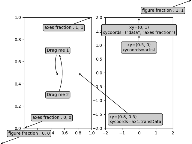
Weitere Beispiele für Koordinatensysteme

Nachfolgend zeigen wir einige weitere Beispiele für Koordinatensysteme und wie die Position von Annotationen angegeben werden kann.

fig, (ax1, ax2) = plt.subplots(1, 2)

bbox_args = dict(boxstyle="round", fc="0.8")
arrow_args = dict(arrowstyle="->")

# Here we'll demonstrate the extents of the coordinate system and how
# we place annotating text.

ax1.annotate('figure fraction : 0, 0', xy=(0, 0), xycoords='figure fraction',
             xytext=(20, 20), textcoords='offset points',
             ha="left", va="bottom",
             bbox=bbox_args,
             arrowprops=arrow_args)

ax1.annotate('figure fraction : 1, 1', xy=(1, 1), xycoords='figure fraction',
             xytext=(-20, -20), textcoords='offset points',
             ha="right", va="top",
             bbox=bbox_args,
             arrowprops=arrow_args)

ax1.annotate('axes fraction : 0, 0', xy=(0, 0), xycoords='axes fraction',
             xytext=(20, 20), textcoords='offset points',
             ha="left", va="bottom",
             bbox=bbox_args,
             arrowprops=arrow_args)

ax1.annotate('axes fraction : 1, 1', xy=(1, 1), xycoords='axes fraction',
             xytext=(-20, -20), textcoords='offset points',
             ha="right", va="top",
             bbox=bbox_args,
             arrowprops=arrow_args)

# It is also possible to generate draggable annotations

an1 = ax1.annotate('Drag me 1', xy=(.5, .7), xycoords='data',
                   ha="center", va="center",
                   bbox=bbox_args)

an2 = ax1.annotate('Drag me 2', xy=(.5, .5), xycoords=an1,
                   xytext=(.5, .3), textcoords='axes fraction',
                   ha="center", va="center",
                   bbox=bbox_args,
                   arrowprops=dict(patchB=an1.get_bbox_patch(),
                                   connectionstyle="arc3,rad=0.2",
                                   **arrow_args))
an1.draggable()
an2.draggable()

an3 = ax1.annotate('', xy=(.5, .5), xycoords=an2,
                   xytext=(.5, .5), textcoords=an1,
                   ha="center", va="center",
                   bbox=bbox_args,
                   arrowprops=dict(patchA=an1.get_bbox_patch(),
                                   patchB=an2.get_bbox_patch(),
                                   connectionstyle="arc3,rad=0.2",
                                   **arrow_args))

# Finally we'll show off some more complex annotation and placement

text = ax2.annotate('xy=(0, 1)\nxycoords=("data", "axes fraction")',
                    xy=(0, 1), xycoords=("data", 'axes fraction'),
                    xytext=(0, -20), textcoords='offset points',
                    ha="center", va="top",
                    bbox=bbox_args,
                    arrowprops=arrow_args)

ax2.annotate('xy=(0.5, 0)\nxycoords=artist',
             xy=(0.5, 0.), xycoords=text,
             xytext=(0, -20), textcoords='offset points',
             ha="center", va="top",
             bbox=bbox_args,
             arrowprops=arrow_args)

ax2.annotate('xy=(0.8, 0.5)\nxycoords=ax1.transData',
             xy=(0.8, 0.5), xycoords=ax1.transData,
             xytext=(10, 10),
             textcoords=OffsetFrom(ax2.bbox, (0, 0), "points"),
             ha="left", va="bottom",
             bbox=bbox_args,
             arrowprops=arrow_args)

ax2.set(xlim=[-2, 2], ylim=[-2, 2])
plt.show()